ism3d.arts: model artificial sources in different shapes
Setup
We first import essential API functions / modules from ism3d and other libraries
Used ISM3D Functions:
im3d.logger.logger_configim3d.logger.logger_status
[8]:
nb_dir=_dh[0]
os.chdir(nb_dir+'/../output/mockup')
sys.path.append(nb_dir)
from notebook_setup import *
%matplotlib inline
#%config InlineBackend.figure_format = "png" # ‘png’, ‘retina’, ‘jpeg’, ‘svg’, ‘pdf’.
%reload_ext wurlitzer
%reload_ext memory_profiler
%reload_ext line_profiler
#ism3d.logger_config(logfile='ism3d.log',loglevel='INFO',logfilelevel='INFO',log2term=False)
ism3d.logger_config(logfile='ism3d.log',loglevel='DEBUG',logfilelevel='DEBUG',log2term=False)
print(''+ism3d.__version__)
print('working dir: {}\n'.format(os.getcwd()))
0.3.dev1
working dir: /Users/Rui/Resilio/Workspace/projects/ism3d/models/output/mockup
2D Analytic Model Rendering
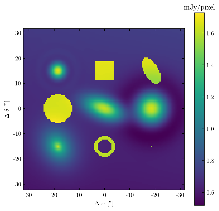
We read the model configuration from a parameter file following the INI file format). Then we render it into a specifield WCS system for visulization purposes.
A 2D analytical object has the following properties: + the same spatial distribution at different frequency (thought the integrated flux can vary (described by frequency-depdendent fluxscale vector) + no inclination or object thickness, just flat “on-sky” prescription although there is a angular-physicallength transformation + 3D analytical model can be easily rendered into a regular grid (specified by WCS) and then rendered into UV data using the grid-to-sparse transform from FNUFFT.
Used ISM3D Functions:
ism3d.utils.meta.create_headerism3d.interface.read_inpism3d.interface.inp_to_modism3d.modeling.model.model_realizeism3d.simxy.render.render_apmodel2d
[2]:
header=create_header(naxis=[128,128,120],
objname='arts.models',
crval=[189.2933333,62.3711111,45535299115.90349],
cdelt=[-0.5/3600,0.5/3600,2000013.13785553])
inpfile='../../input/mockup_apmodel2d.ini'
inp_dict=read_inp(inpfile)
mod_dict=inp_to_mod(inp_dict)
model_name='mockup5'
from ism3d.simxy.render import render_apmodel2d as xy_render_apmodel2d
out=0
for obj in mod_dict:
plane,fluxscale=xy_render_apmodel2d(mod_dict[obj],WCS(header),normalize=False)
#print(obj,mod_dict[obj]['sbProf'],plane.sum(),np.max(plane),fluxscale[0].value)
out=out+plane*fluxscale[0].value
fits.writeto('mockup_arts.fits',out,header,overwrite=True)
im_grid(out*1e3,header,offset=True,units=['mJy/pixel'],
titles=None,nxy=(1,1),figsize=(5,5),
figname='mockup_arts.pdf',showplot=True)
<Figure size 432x288 with 0 Axes>
3D Sparse Model Rendering
Here, we render a model composed of three “sparse-array” 3D objectes/ The mapping destination is again specified by a WCS system and we visulize the results as an channel map animation.
A 3D “cloudlet” object has the following properties: + each object is described by a particle collection (sparse array). the equal-weight particle PDF and their kimeatical properties follow specified analytical prescriptions. Basically, it’s a particle-based representation of the model object in terms of it’s morphological and kinmeatic properties. + inclination and object thickness are incorperated, plus several transformation from the model system to on-sky system: orientation > physical-to-sky
Note: + resolved line emission can only be described by 3D sparse model + A continue object stil be represented by a 3D sparse model. + 3D sparse model can be directly rendered into UV data using the sparse-to-sparse transform from FNUFFT
Used ISM3D Functions:
ism3d.utils.meta.create_headerism3d.interface.read_inpism3d.interface.inp_to_modism3d.modeling.model.model_realizeism3d.simxy.render.render_apmodel2d
[3]:
header=create_header(naxis=[128,128,120],
objname='arts.models',
crval=[189.2933333,62.3711111,45535299115.90349],
cdelt=[-0.5/3600,0.5/3600,2000013.13785553])
inpfile='../../input/mockup_spmodel3d.ini'
inp_dict=read_inp(inpfile)
mod_dict=inp_to_mod(inp_dict)
model_name='mockup5'
out=0
for obj in mod_dict:
cube=xy_render_spmodel3d(mod_dict[obj],WCS(header))
#print(obj,mod_dict[obj]['sbProf'],plane.sum(),np.max(plane),fluxscale[0].value)
out=out+cube
#pprint(mod_dict) # the sparse models have been added as caching keywords clouds_wt/clouds_loc
fits.writeto('mockup_arts3d.fits',out,header,overwrite=True)
add the 3D model realization
add the 3D model realization
add the 3D model realization
add the 3D model realization
add the 3D model realization
[4]:
nchan=header['NAXIS3']
stepchan= int(np.maximum(np.floor(int(nchan/20)),1))
vmax=np.nanmax(out)
vmin=np.nanmin(out)
fignames=[]
for ichan in range(0,nchan,stepchan):
#clear_output(wait=True)
figname='mockup_arts3d.chmap/ch{:03d}'.format(ichan)+'.pdf'
images=[out[ichan,:,:]]
titles=['arts3d['+'{}'.format(ichan)+']']
im_grid(images*1000,header,offset=True,units=['mJy/pixel'],
titles=titles,nxy=(1,1),figsize=(10,10),figname=figname,vmins=[vmin],vmaxs=[vmax]) ;
fignames.append(figname)
make_gif(fignames,'mockup_arts3d.chmap/chmap.gif')
show_gif('mockup_arts3d.chmap/chmap.gif')
[4]:

<Figure size 432x288 with 0 Axes>
[5]:
#clouds_loc=mod_dict['contdisk4']['clouds_loc']
#x=clouds_loc.x.value
#y=clouds_loc.y.value
#z=clouds_loc.z.value
#N = 1000
#x, y, z = np.random.normal(0, 1, (3, N))
#fig = ipv.figure()
#scatter = ipv.scatter(x, y, z,size=0.2,marker='sphere')
#ipv.show()
Volume Rendering based on IPyvolume
[6]:
cube,edges=xy_render_spmodel3d_xyz(mod_dict['contdisk4'])
fits.writeto('xyz.fits',cube,overwrite=True)
cube=fits.getdata('xyz.fits')
fig = ipv.figure()
ipv.quickvolshow(cube)
#ipv.volshow(cube,level=[0.1,0.5,0.9])
#ipv.view(20,20)
#ipv.show()
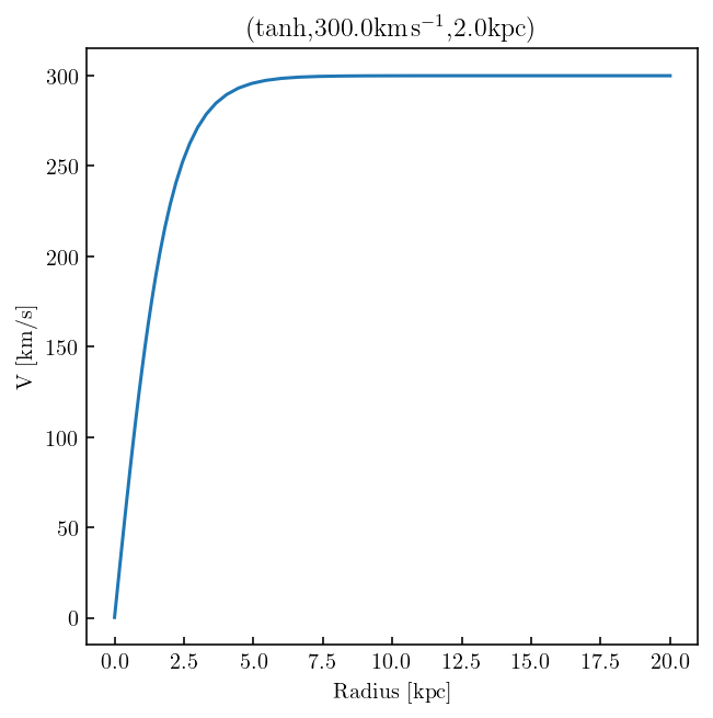
[7]:
inpfile='../../input/mockup_spmodel3d.ini'
inp_dict=read_inp(inpfile)
mod_dict=inp_to_mod(inp_dict)
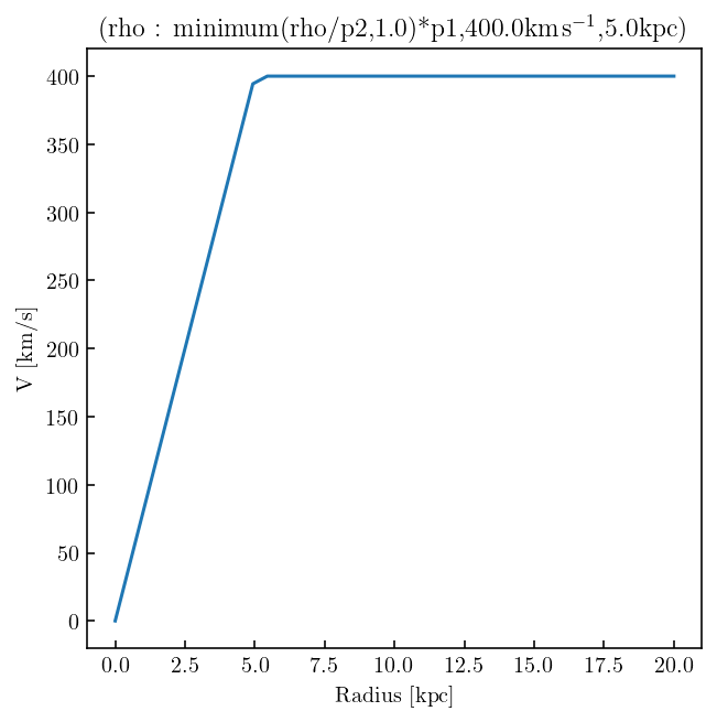
plt_rcProf(mod_dict['co21disk1']['rcProf'],showplot=True)
plt_rcProf(mod_dict['co21disk2']['rcProf'],showplot=True)
[ ]:
[ ]: